Advanced Operator Panels Items
The following explanations assume that you are familiar with the basics of Using Operator Panels. Use the Operator Panel Example model from the file menu to access the model used here. This tutorial covers the following operator panel items: 2D Area Input, 2D Graph Viewer, 3D Viewer

2D Area Input
The 2D area input item allows to user to move a cursor within a rectangular or quadratic area and thereby select two input values at the same time.
For example, this input item can be used to model a steering stick or joystick.
The area input works for three different types: boolean, int, and double.
The following picture shows the simulation view of the area input item for each type.
During the simulation the black circular cursor can be moved by dragging the mouse across the input area.
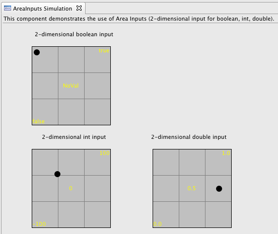
Double-clicking in one of the grid areas makes the cursor jump to the minimum, center, and maximum value of the area input.
For example, the center grid of the int type item makes the cursor jump to the (0,0) location, while the upper-right grid makes it jump to the (100, 100) location.
For the boolean type item the exact location of the cursor is not relevant, only the grid is evaluated and interpreted as one of the three possible port values: false, NoVal, or true.
For the int and double type item the exact position of the cursor is interpreted with the respective interval (-100 to 100, or 0.0 to 1.0).
The following picture shows the property section of the area input item:
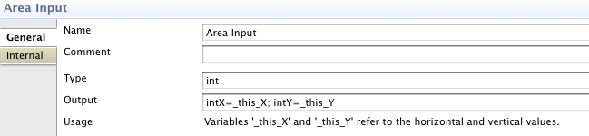
In the type field the item type is specified. Enter boolean, int, or double here.
In the output field the port values are assigned by using the user input stored in the _this_X and _this_Y variables.
Here, you can scale the input to the values required by the application or you can use the raw value and add another component to your system, which does the scaling. Note that the display of the area input will always show the values depicted above, not the values you compute for output ports. Therefore, the second option is possibly the more intuitive one, since the user will see his entered values directly on the output channels.
2D Graph Viewer
The 2D Graph Viewer output item allows to plot numeric values with an oscilloscope-like display. The following picture shows the simulation output of the 2D graph viewer item. Note that it may take a few seconds to initialize the OpenGL font, the first time you open this simulation view.
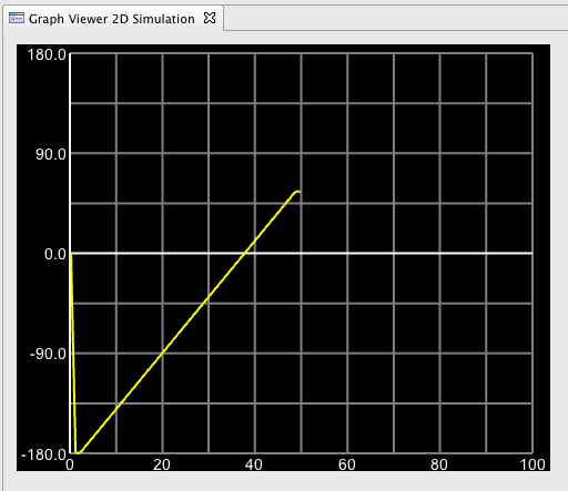
The input to this component over time is a counter from 0 to 360 degree, which is plotted in the graph view from -180 to +180. The following picture of the property section of the 2D graph viewer item shows how this output is computed:

In the type field the item type is specified. Enter boolean, int, or double here.
In the sample value field the displayed value is computed from the input port values.
The samples per grid value specifies how many time steps should be displayed in each horizontal section of the grid.
The levels per grid value specifies how many value units should be displayed in each vertical section of the grid.
In the line color field you can specify the red, green, and blue color component of the line color (each value is between 0.0 and 1.0).
In the number of horizontal grids field you specify how many grid fields should be displayed horizontally. Adapt this value to the size you have chosen for the panel item. Enter one to get rid of the grid.
In the number of vertical grids field you specify how many grid fields should be displayed vertically above and below the horizontal axis. In the example there are four grids above and four below the origin line. Again, enter one to get rid of the grid.
3D Object Viewer
The 3D Object Viewer output item allows to render simple 3D scenes with imported meshes and translations, rotations, and scalings computed from input port values. The 3D Viewer comes with its own editor, which you can access by double-clicking the item in the operator panel editor or the model navigator.The following picture is showing the example scene during the simulation:
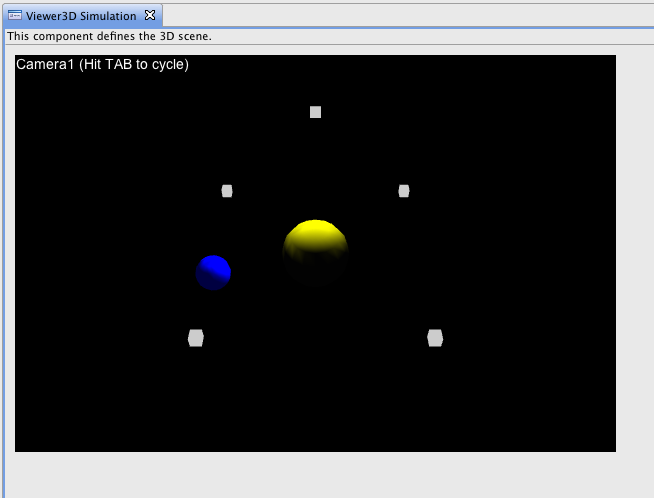
The scene shows the following objects from the Camera1 perspective:
- a yellow sphere in the the center
- a blue sphere, which circles the yellow one in the X-Y-plane
- four white cubes, which are added as references for the X-Y-plane
- another white cube, which shows the location of the light source
- a hint to hit the TAB key to cycle through the cameras
The scene contains two cameras: the static Camera1 (looking at the origin from a small distance along the positive Y axis) and the moving Camera2 (looking a the origin from a small distance along the X axis and pitching from -20 to 20 degree below and above the X-Y-plane). The whole animation is driven by a counter component, which counts from zero to 360 and back to zero. From this input value all object positions are derived using rotation object nodes (see below).
The following picture shows the scene editor of the example.
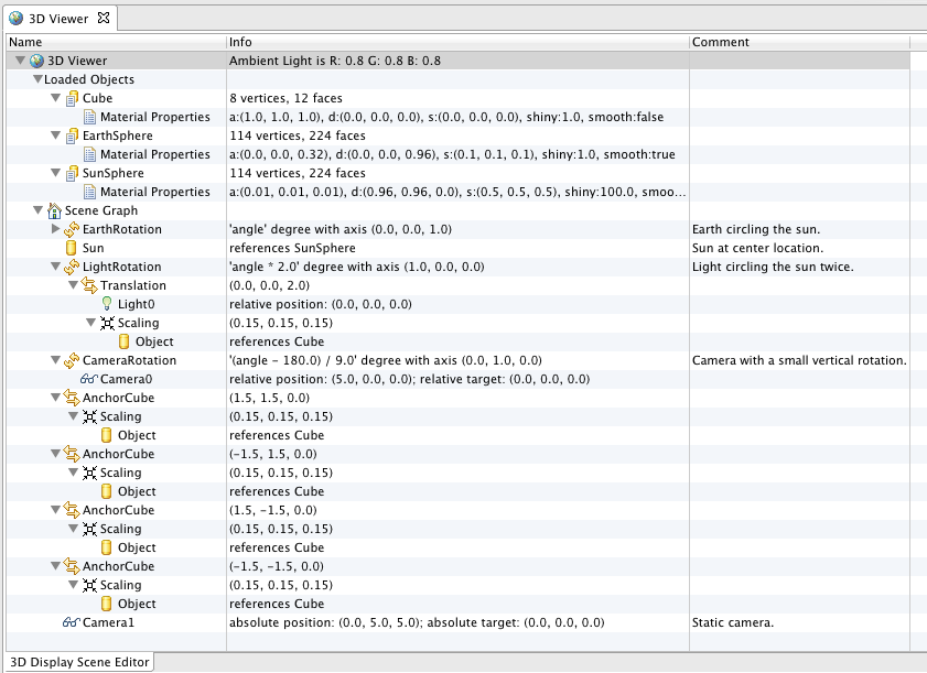
You can drag objects and display nodes from the library view to scene editor tree.

Note that you have to drop Cubes and Spheres onto the 3D Viewer tree entry, not the loaded objects entry. You can replace the cube or sphere objects with arbitrary meshes from 3D modeling tools (like Blender) as described below.
World Coordinates
The whole scene uses a world coordinate system with the positive Z axis being the upward direction of cameras. In other words the X-Y-plane is the surface of the scene world. Camera perspective is fixed to a 45 degree field of view with the near distance set to 0.5 and the far distance set to 400.0.
Cameras and Lights
Each scene needs a least one camera, which means that the scene graph must contain at least one Camera Node. Cameras are defined by specifying an eye position and a look target location, which may not be the same (i.e. they define a vector). If you want the camera to be translated and/or rotated, you should set either the eye or the target location to the origin and the other one unit away in either X or Y direction. See Camera0 in the example for moving camera with fixed target location.

The scene viewer can be used with or without using the OpenGL light engine. You can switch the use of light using the property section of the 3D Viewer tree item. There you can also set the ambient light intensity when the light is turned on. If the light is turned off, the ambient component of the material of loaded objects will be used as color (see next section).
A light source can be specified by adding a Light Node to the scene graph. There is a maximum of 8 lights currently supported. With the property section you can specify the properties of the light source, in particular, its ambient, diffuse, and specular intensities/colors as well as the attenuation coefficients.
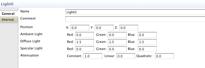
Note that lights can also be positioned in the scene by using transformations (see below).
Objects and Materials
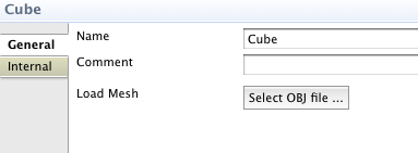
Objects in the scene are built from meshes (i.e. sets of triangles). More complex objects can be loaded from external files using the button from the property. See below for information on how to export proper meshes from the Blender 3D modeling tool.
Each object's triangles are associated with a material, which describes the objects reaction to light sources. These values are imported when the object is loaded, but can be changed in the editor.
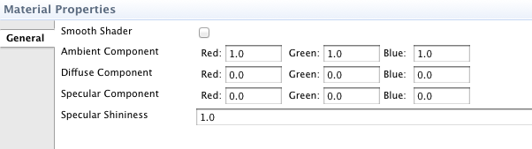
If the light engine is disabled the ambient component of the material is used as color. Each loaded object is instantiated in the scene graph by adding Object Nodes. The property section of the object node references a loaded object by name. Note that loaded objects can be used by multiple object nodes with each node possibly being transformed differently. For example, the white cube is used five times in the tutorial model.
Transformations: Translation, Rotation, and Scaling
You can move or animate objects by specifying transformation nodes. Each such nodes applies its transformation to the model view matrix of OpenGL before its sub-components are processed. There transformations can be chained to allow to draw any object at any location, rotation and size. Furthermore, the values for the transformation can be computed from input port values, which allows animation.
The following picture shows the rotation node properties for the blue sphere (the rotation angle is taken from the input port angle):
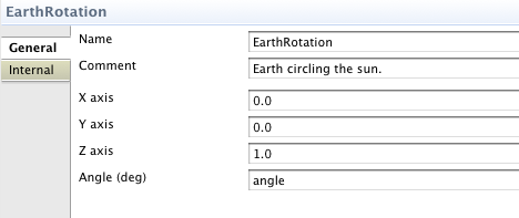
The property sections of translations and scalings work similar. The X, Y, and Z values can also be computed from input port values.
Using Blender to replace Object meshes.
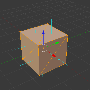
When using Blender to produce the objects to be shown in the 3D Viewer make sure you trianlges and all the normal vectors point in the right direction. Here is an example picture from the default cube with normals pointing outward.
Before you can import your mesh in the 3D viewer, you must export it from Blender into the Wavefront format (.OBJ object and .MTL material files). Make sure the edges, normals and materials are exported and the mesh has triangulated faces (if you haven't done so during editing). Here is an example of the export options that were tested for AF3.
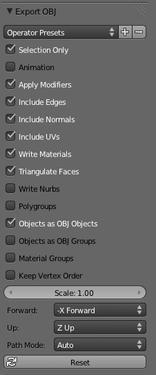
You are advised to export your mesh with correct up axis.